Documentation

Interictal epileptiform discharges (IEDs), also referred to as ”spikes”, are a characteristic of the epileptic brain that are recognizable as large transient events in the electroencephalogram of patients living with epilepsy [1]. Whereas, for clinicians, IEDs can provide valuable information about the epileptogenic zone, for researchers, they can also be a source of noise and need to be excluded, such as in [2] where Cusinato and Alnes et al. studied how the human brain processes sounds. Regardless of the context, the localization of IEDs in EEG recordings is a very time-consuming task.

This package aims to contribute to this issue by building on an algorithm previously developed by Baud et al. [3] that employs nonnegative matrix factorization (NMF) to automatically detect IEDs, an unsupervised machine-learning algorithm that produces a lower-dimensional approximation of the input.

It is important to note, that the algorithm used by this package is optimized for and was solely tested on intracranial EEG (iEEG) recordings. Intracranial EEG is an invasive technique with implanted electrodes that is used for clinical monitoring, e.g. to identify the epileptogenic zone and prepare for epilepsy surgery. The primary characteristic of iEEG is that it provides high spatial and temporal resolution of the electrical activity in the brain, which makes it a valuable resource for neuroscientific research as well [4].

Nonnegative Matrix Factorization

Nonnegative Matrix Factorization (NMF) is a machine-learning algorithm used to decompose an original data matrix into two lower-rank matrices. As such it resembles other matrix decomposition algorithms, such as Principal Component Analysis (PCA), Linear Discriminant Analysis (LDA), and Independent Component Analysis (ICA), whose purpose is to reduce the dimensionality of the original data and to identify the underlying patterns, principal components or latent variables that make up the observed data. The unique characteristic of NMF is that it imposes nonnegativity constraints on the values of the factorized matrices, which only allow for additive combinations and thus result in a parts-based representation of the original data. This characteristic improves the interpretability of the results [5, 6]. In many real-world applications, such as image processing, text analysis or gene data analysis, the presence of negative values in both the original data and the latent variables is physically meaningless. This limits the application scenarios for methods like PCA and ICA [5, 7]. In [6], Lee and Seung, using image data, showed that the decomposition of human faces performed by NMF results in a range of facial parts, such as noses, mouths, and eyes, corresponding to the different parts making up the whole. By contrast, when applied to the same data set, PCA yields a set of prototypical eigenfaces that by linear combination approximates the original data.

The basic mechanism of NMF, illustrated in Fig. 1, is that it approximates an original data matrix by the linear combination of two nonnegative lower-rank matrices

\[V ≈W ×H\]

Here, \(V\) is a \(M × N\) matrix incorporating the original data in terms of features (rows) and samples (columns). \(W\) is a \(M × K\) matrix, whose K columns are called basis vectors and represent the latent variables, expressed by the same features as the observed data. \(H\) is a \(K × N\) matrix whose columns are the encodings of the samples [6, 8].

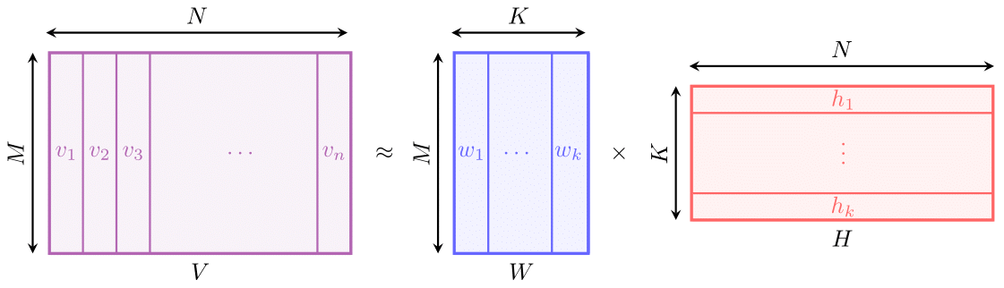
Fig. 1 Conceptual diagram of Nonnegative Matrix Factorization (NMF)

A further result reported by Lee and Seugn is that both the basis vectors and the encodings contain numerous vanishing coefficients, meaning that both the basis images and encodings are sparse [6]. The basis images contain several versions of different facial parts that are in different locations and have different forms, accounting for their sparsity. The sparsity in the image encodings is explained by the fact that all parts are used by at least one image, but no image uses all parts. In [8], Brunet et al. introduced NMF as a means of reducing the dimension of expression data from thousands of genes to a small number of metagenes. By combining NMF with consensus clustering, a model-selection algorithm developed in [9] and adding a quantitative evaluation to assess the robustness of a given decomposition, they were able to identify distinct molecular patterns and cluster samples into the different metagenes. In their model, the data matrix consists of the gene expression levels of–expressed in terms of the variables introduced above–\(M\) genes in \(N\) samples. The decomposition results in a matrix \(W\) , consisting of \(K\) metagenes, each expressed in terms of the \(M\) genes, and an \(H\) matrix whose \(N\) columns represent the metagene expression pattern of each individual sample. Translating NMF into the context of EEG data while using the analogous terminology, NMF decomposes a set of EEG signals into a small number of EEG metapatterns that make up these signals. The original data matrix \(V\) contains the measurements of the electrical activity in the brain from \(M\) different electrodes along \(N\) different time points. The \(K\) columns of W then represent the EEG metapatterns contained in the original signals, expressed in terms of the different brain activity patterns captured by the \(M\) electrodes, while the \(N\) columns of \(H\) represent the activation level of each metapattern at each point in time.

Extensions

The methodology used in this package employs consensus clustering [9] to automatically determine the optimal rank of the decomposition, following the example of Brunet et al. [8] described in the previous section.

Additionally, the package offers a modified version of the NMF algorithm, which attempts to further exploit the spatiotemporal features of the EEG signals by integrating sparseness constraints. The method uses a model of sparseness introduced by Hoyer [10] who defined sparseness based on a relation between the \(L_1\) norm and the \(L_2\) norm

\[sparseness(x) = \frac{\sqrt{n} - (\sum | x_i |) / \sqrt{\sum x_{i}^2}}{\sqrt{n} - 1},\]

where \(x\) is a vector and \(n\) is the dimensionality of \(x\). This function has the advantage of interpolating smoothly in the interval [0, 1] and evaluating to 0 if and only if all elements of \(x\) are equal and to 1 if and only if \(x\) contains a single non-zero element. In our model, we impose sparseness constraints on individual basis vectors, i.e. the columns of \(W\). We can then define the sparseness of a single basis vector \(w_i\) as

\[sparseness(w_i) = \frac{\sqrt{n} - (\sum | w_{ij} |) / \sqrt{\sum w_{ij}^2}}{\sqrt{n} - 1},\]

where \(w_{ij}\) is the \(j^{th}\) element of the \(i^{th}\) basis vector \(w_i\).

Glossary

Here, we quickly present the most important terminologies used in the library.

Basis Function

A basis function refers to a column of the \(W\) matrix and represents an EEG metapattern, expressed in terms of the different brain activity patterns captured by the employed electrodes. They are represented in the library by the BasisFunction object.

Activation Function

An activation function refers to a single row of the \(H\) matrix and contains the activation levels of a given metapattern at each point in time. They are represented by the ActivationFunction object.

Limitations

The default algorithm ran by means of the SpikeDetectionPipeline employs a simple K-Means clustering to split the returned activation functions into those coding for a certain EEG pattern and those coding for noise and sorts them starting with the noisy functions. However, there is no functionality that is guaranteed to find which of the activation functions exactly codes for spikes. Therefore, it is recommended to use additional tools that allow the visualization of the activation functions and their respective event periods.

References

[1]

Marco de Curtis and Giuliano Avanzini. “Interictal spikes in focal epileptogenesis”. Progress in Neurobiology 63, no.5 (2001): 541-567.

[2]

Riccardo Cusinato, Sigurd L. Alnes, Ellen van Maren, Ida Boccalaro, Debora Ledergerber, Antoine Adamantidis, Lukas L. Imbach, Kaspar Schindler, Maxime O. Baud, and Athina Tzovara. Intrinsic neural timescales in the temporal lobe support an auditory processing hierarchy. Journal of Neuroscience, 43(20):3696–3707, 2023.

[3]

Maxime O. Baud, Jonathan K. Kleen, Gopala K. Anumanchipalli, Liberty S. Hamilton, Yee-Leng Tan, Robert Knowlton, and Edward F. Chang. Unsupervised learning of spatiotemporal interictal discharges in focal epilepsy. Neurosurgery, 83(4), 2018.

[4]

Elizabeth L Johnson, Julia W Y Kam, Athina Tzovara, and Robert T Knight. Insights into human cognition from intracranial eeg: A review of audition, memory, internal cognition, and causality. Journal of Neural Engineering, 17(5):051001, oct 2020.

[5]

Yu-Xiong Wang and Yu-Jin Zhang. Nonnegative matrix factorization: A comprehensive review. IEEE Transactions on Knowledge and Data Engineering, 25(6):1336–1353, 2013.

[6]

Daniel D. Lee and H. Sebastian Seung. Learning the parts of objects by non-negative matrix factorization. Nature, 401(6755):788–791, Oct 1999.

[7]

Jiangzhang Gan, Tong Liu, Li Li, and Jilian Zhang. Non-negative Matrix Factorization: A Survey. The Computer Journal, 64(7):1080–1092, 07 2021.

[8]

Jean-Philippe Brunet, Pablo Tamayo, Todd R. Golub, and Jill P. Mesirov. Metagenes and molecular pattern discovery using matrix factorization. Proceedings of the National Academy of Sciences, 101(12):4164–4169, 2004.

[9]

Stefano Monti, Pablo Tamayo, Jill Mesirov, and Todd Golub. Consensus clustering: A resampling- based method for class discovery and visualization of gene expression microarray data. Machine Learning, 52(1):91–118, Jul 2003.

[10]

Patrik O Hoyer. ‘Non-negative matrix factorization with sparseness constraints’ Journal of Machine Learning Research 5:1457-1469, 2004.